Welcome to the exercises on variance, mean deviation, and standard deviation! In this series of exercises, we will explore fundamental concepts in statistics that will help us understand the dispersion and variability of a data set.

Variance, mean deviation, and standard deviation are statistical measures that allow us to quantify the dispersion or variability of a data set with respect to its mean. These measures are especially useful for understanding how dispersed or grouped the values of a data set are and how they are distributed around their central value.

Get ready to strengthen your skills in statistics and discover the fascinating world of data analysis. Let's get started!

Score:

Find the mean deviation, the variance, and the standard deviation of $\text{[math]}$ .

Solution

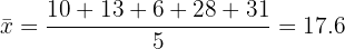
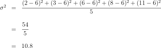
1 We compute the mean for the series of numbers $\text{[math]}$ , with n=5=N. We have the following computations.

$\text{[math]}$

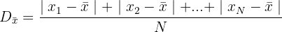
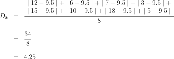
2 We compute the value of the mean deviation.

$\text{[math]}$

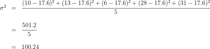
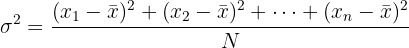
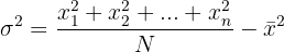
3 Now, we compute the value of the variance.

$\text{[math]}$

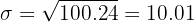
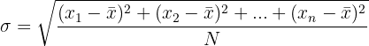
4 And finally, we compute the value of the standard deviation.

$\text{[math]}$

Find the mean deviation, the variance, and the standard deviation of the following series of numbers:

a 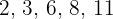$\text{[math]}$ .

b $\text{[math]}$ .

Solution

a For the series of numbers $\text{[math]}$ with we have the following calculations:

For the mean deviation, we first need to compute the mean.

$\text{[math]}$

We compute the value of the mean deviation.

$\text{[math]}$

Now, we compute the value of the variance.

$\text{[math]}$

And finally, we compute the value of the standard deviation.

$\text{[math]}$

b For the series of numbers $\text{[math]}$ with $\text{[math]}$ , we have the following computations.

For the mean deviation, we first need to compute the mean.

$\text{[math]}$

Then, we compute the value of the mean deviation.

$\text{[math]}$

Now, we compute the value of the variance.

$\text{[math]}$

And finally, we compute the value of the standard deviation.

$\text{[math]}$

Find the variance and the standard deviation of $\text{[math]}$ .

Solution

1 We build the frequency table and include the product of the variable by its absolute frequency $\text{[math]}$ to compute the mean, and the product of the squared variable by its absolute frequency $\text{[math]}$ to compute the variance and the standard deviation.

$\text{[math]}$	$\text{[math]}$	$\text{[math]}$	$\text{[math]}$
5	3	15	75
6	2	12	72
7	2	14	98
8	2	16	128
9	3	27	243
10	2	20	200
13	1	13	169
	15	117	985

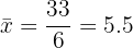
2 We compute the arithmetic mean.

$\text{[math]}$

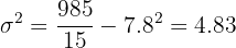
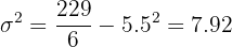
3 We compute the variance.

$\text{[math]}$

4 We compute the standard deviation.

$\text{[math]}$

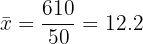
A pediatrician obtained the following table about the age (in months) of 50 children from their practice at the time they walked for the first time. Compute the variance.

Months	Children
9	1
10	4
11	9
12	16
13	11
14	8
15	1

Solution

We complete the table with:

1 The product of the variable by its absolute frequency $\text{[math]}$ to compute the mean.

2 The product of the squared variable by its absolute frequency $\text{[math]}$ to compute the variance and the standard deviation.

$\text{[math]}$	$\text{[math]}$	$\text{[math]}$	$\text{[math]}$
9	1	9	81
10	4	40	400
11	9	99	1089
12	16	192	2304
13	11	143	1859
14	8	112	1568
15	1	15	225
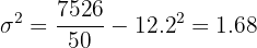
	50	610	7526

Review these concepts with our math tutor.

We compute the arithmetic mean.

$\text{[math]}$

We compute the variance.

$\text{[math]}$

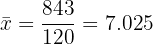
The result of rolling two dice 120 times is given by the table. Compute the variance.

Sums	Times
2	3
3	8
4	9
5	11
6	20
7	19
8	16
9	13
10	11
11	6
12	4

Solution

1 We add the columns $\text{[math]}$

x_i	f_i	x_i * f_i	x_i^2 * f_i
2	3	6	12
3	8	24	72
4	9	36	144
5	11	55	275
6	20	120	720
7	19	133	931
8	16	128	1024
9	13	117	1053
10	11	110	1100
11	6	66	726
12	4	48	576
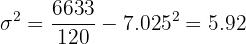
	120	843	6633

2 We compute the arithmetic mean.

$\text{[math]}$

3 We compute the variance.

$\text{[math]}$

Compute the variance of a statistical distribution given by the following table.

	$\text{[math]}$
[10, 15)	3
[15, 20)	5
[20, 25)	7
[25, 30)	4
[30, 35)	2

Solution

1 We add the columns $\text{[math]}$

	$\text{[math]}$	$\text{[math]}$	$\text{[math]}$	$\text{[math]}$
[10, 15)	12.5	3	37.5	468.75
[15, 20)	17.5	5	87.5	1,531.25
[20, 25)	22.5	7	157.5	3,543.75
[25, 30)	27.5	4	110	3,025
[30, 35)	32.5	2	65	2,112.5
		21	457.5	10,681.25

2 We compute the mean.

$\text{[math]}$

3 We compute the variance.

$\text{[math]}$

Compute the variance of the distribution in the table.

	$\text{[math]}$	$\text{[math]}$	$\text{[math]}$	$\text{[math]}$
[10, 20)	15	1	15	225
[20, 30)	25	8	200	5,000
[30, 40)	35	10	350	12,250
[40, 50)	45	9	405	18,225
[50, 60)	55	8	440	24,200
[60, 70)	65	4	260	16,900
[70, 80)	75	2	150	11,250
		42	1,820	88,050

Solution

1 We compute the mean.

$\text{[math]}$

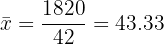
2 We compute the variance.

$\text{[math]}$

The heights of the players on a basketball team are given by the table. Compute the variance.

Height	Number of Players
[5.6ft, 5.7ft)	1
[5.7ft, 5.9ft)	3
[5.9ft, 6.1ft)	4
[6.1ft, 6.2ft)	8
[6.2ft, 6.4ft)	5
[6.4ft, 6.6ft)	2

Solution

1 We complete the table with the columns $\text{[math]}$

	$\text{[math]}$	$\text{[math]}$	$\text{[math]}$	$\text{[math]}$	$\text{[math]}$
[5.6ft, 5.7ft)	5.7ft	1	1	5.7ft	9.8ft
[5.7ft, 5.9ft)	5.8ft	3	4	17.5ft	31ft
[5.9ft, 6.1ft)	6ft	4	8	24ft	43.7ft
[6.1ft, 6.2ft)	6.2ft	8	16	49.2ft	92.3ft
[6.2ft, 6.4ft)	6.3ft	5	21	31.6ft	60.8ft
[6.4ft, 6.6ft)	6.5ft	2	23	13ft	25.6ft
		23		140.8ft	263.2ft

2 We compute the mean.

$\text{[math]}$

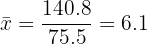
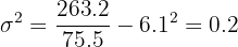
3 We compute the variance.

$\text{[math]}$

Given the statistical distribution, compute the variance.

	$\text{[math]}$
[0, 5)	3
[5, 10)	5
[10, 15)	7
[15, 20)	8
[20, 25)	2
[25, ∞)	6

Solution

1 We complete the table with the columns $\text{[math]}$

	$\text{[math]}$	$\text{[math]}$	$\text{[math]}$
[0, 5)	2.5	3	3
[5, 10)	7.5	5	8
[10, 15)	12.5	7	15
[15, 20)	17.5	8	23
[20, 25)	22.5	2	25
[25, $\text{[math]}$ )		6	31
		31

2 It is not possible to compute the mean, because it is not possible to find the class midpoint of the last interval.

3 If there is no mean, it is not possible to compute the variance.

Consider the following data: $\text{[math]}$ . Then:

a Compute its mean and its variance.

b If we multiply all the previous data by $\text{[math]}$ , what will the new mean and variance be?

Solution

We complete the table with the column $\text{[math]}$

$\text{[math]}$	$\text{[math]}$
2	4
3	9
4	16
6	36
8	64
10	100
33	229

1 Mean and variance:

$\text{[math]}$

2 If all the values of the variable are multiplied by a number, the mean is multiplied by $\text{[math]}$ and the variance is multiplied by the square of that number.

$\text{[math]}$

Summarize with AI:

Did you like this article? Rate it!

5.00 (2 Note(n))

Agostina Babbo

Agostina Babbo is an English and Italian to Spanish translator and writer, specializing in product localization, legal content for tech, and team sports—particularly handball and e-sports. With a degree in Public Translation from the University of Buenos Aires and a Master's in Translation and New Technologies from ISTRAD/Universidad de Madrid, she brings both linguistic expertise and technical insight to her work.

Exercises and Problems on Variance, Mean Deviation, and Standard Deviation

Understanding the Median: Definition and Calculation Methods

Percentiles: What Are They and How to Calculate Them?

Solved Frequency Exercises