Statistics is a fundamental tool for analyzing and interpreting data across various disciplines, from social sciences to engineering. Understanding statistical concepts and knowing how to apply them correctly is crucial for making informed decisions based on data.
This section of solved exercises is designed to help consolidate the theoretical knowledge acquired in statistics topics. Through practice with real problems, the goal is to develop analytical skills and strengthen the ability to solve common and complex statistical situations.
Indicate which variables are qualitative and which are quantitative
- Favorite food.
- Career you like.
- Number of goals scored by your favorite team in the last season.
- Number of students in your school.
- Eye color of your classmates.
- Intelligence coefficient of your classmates.
- Favorite food. Qualitative
- Profession you like. Qualitative
- Number of goals scored by your favorite team in the last season. Quantitative
- Number of students in your school. Quantitative
- Eye color of your classmates. Qualitative
- Intelligence coefficient of your classmates. Quantitative
Indicate which of the following variables are discrete and which are continuous:
- Number of shares sold each day on the stock exchange.
- Temperatures recorded each hour at an observatory.
- Duration period of a car.
- The diameter of the wheels of several cars.
- Number of children in 50 families.
- Annual census of American people.
- Number of shares sold each day on the stock exchange. Discrete
- Temperatures recorded each hour at an observatory. Continuous
- Duration period of a car. Continuous
- The diameter of the wheels of several cars. Continuous
- Number of children in 50 families. Discrete
- Annual census of American people. Discrete
Classify the following variables as qualitative or quantitative, and as discrete or continuous:
- The nationality of a person.
- Number of gallons of water contained in a tank.
- Number of books on a bookshelf.
- Sum of points obtained when rolling a pair of dice.
- The profession of a person.
- The area of the different tiles of a building.
- The nationality of a person. Qualitative
- Number of gallons of water contained in a tank. Quantitative and continuous
- Number of books on a bookshelf. Quantitative and discrete
- Sum of points obtained when rolling a pair of dice. Quantitative and discrete
- The profession of a person. Qualitative
- The area of the different tiles of a building. Quantitative and continuous
The scores obtained by a group on a test were:

Construct the frequency distribution table and draw the frequency polygon.
| Value | Tally | Frequency | Cumulative Frequency | Relative Frequency | Cumulative Relative Frequency |
|---|---|---|---|---|---|
| 13 | III | 3 | 3 | 0.15 | 0.15 |
| 14 | I | 1 | 4 | 0.05 | 0.20 |
| 15 | V | 5 | 9 | 0.25 | 0.45 |
| 16 | IIII | 4 | 13 | 0.20 | 0.65 |
| 18 | III | 3 | 16 | 0.15 | 0.80 |
| 19 | I | 1 | 17 | 0.05 | 0.85 |
| 20 | II | 2 | 19 | 0.10 | 0.95 |
| 22 | I | 1 | 20 | 0.05 | 1 |
| 20 |
In the fourth column we place the cumulative frequency  .
.
In the first cell we place the first absolute frequency. In the second cell we add the value of the previous cumulative frequency plus the corresponding absolute frequency, and so on until the last, which must be equal to  .
.
In the fifth column we place the relative frequencies  , which are the result of dividing each absolute frequency by
  .
.
In the sixth column we place the cumulative relative frequency  .
.
In the first cell we place the first relative frequency. In the second cell we add the value of the previous cumulative relative frequency plus the corresponding cumulative relative frequency, and so on until the last, which must be equal to  .
.
Frequency Polygon
On the x-axis are the data values and on the y-axis are the absolute frequencies.
The number of stars of the hotels in a city is given by the following series:

Construct the frequency distribution table and draw the bar diagram.
Steps to construct the frequency distribution table and draw the bar diagram:
| Value | Tally | Frequency | Cumulative Frequency | Relative Frequency | Cumulative Relative Frequency |
|---|---|---|---|---|---|
| 1 | VI | 6 | 6 | 0.158 | 0.158 |
| 2 | XII | 12 | 18 | 0.316 | 0.474 |
| 3 | XVI | 16 | 34 | 0.421 | 0.895 |
| 4 | IIII | 4 | 38 | 0.105 | 1 |
| 38 | 1 |
In the fourth column we place the cumulative frequency .
In the first cell we place the first absolute frequency. In the second cell we add the value of the previous cumulative frequency plus the corresponding absolute frequency, and so on until the last, which must be equal to  .
.
In the fifth column we place the relative frequencies () which are the result of dividing each absolute frequency by .
In the sixth column we place the cumulative relative frequency .
In the first cell we place the first relative frequency. In the second cell we add the value of the previous cumulative relative frequency plus the corresponding cumulative relative frequency, and so on until the last, which must be equal to .
Bar Diagram
On the x-axis are the data values and on the y-axis are the absolute frequencies.
The grades of 50 students were as follows:

Construct the frequency distribution table and draw the bar diagram.
Steps to construct the frequency distribution table and draw the bar diagram:
| Value | Frequency | Cumulative Frequency | Relative Frequency | Cumulative Relative Frequency |
|---|---|---|---|---|
| 0 | 1 | 1 | 0.02 | 0.02 |
| 1 | 1 | 2 | 0.02 | 0.04 |
| 2 | 2 | 4 | 0.04 | 0.08 |
| 3 | 3 | 7 | 0.06 | 0.14 |
| 4 | 6 | 13 | 0.12 | 0.26 |
| 5 | 11 | 24 | 0.22 | 0.48 |
| 6 | 12 | 36 | 0.24 | 0.72 |
| 7 | 7 | 43 | 0.14 | 0.86 |
| 8 | 4 | 47 | 0.08 | 0.94 |
| 9 | 2 | 49 | 0.04 | 0.98 |
| 10 | 1 | 50 | 0.02 | 1.0 |
| 50 | 1 |
In the fourth column we place the cumulative frequency .
In the first cell we place the first absolute frequency. In the second cell we add the value of the previous cumulative frequency plus the corresponding absolute frequency, and so on until the last, which must be equal to  .
.
In the fifth column we place the relative frequencies () which are the result of dividing each absolute frequency by .
In the sixth column we place the cumulative relative frequency .
In the first cell we place the first relative frequency. In the second cell we add the value of the previous cumulative relative frequency plus the corresponding cumulative relative frequency, and so on until the last, which must be equal to .
Bar Diagram
On the x-axis are the data values and on the y-axis are the absolute frequencies.
The weights of 65 employees of a factory are given by the following table:
| Weight | |
|---|---|
| [50, 60) | 8 |
| [60, 70) | 10 |
| [70, 80) | 16 |
| [80, 90) | 14 |
| [90, 100) | 10 |
| [100, 110) | 5 |
| [110, 120) | 2 |
- Construct the frequency table.
- Draw the histogram and frequency polygon.
- Construct the frequency table:
| Interval | Value | Frequency | Cumulative Frequency | Relative Frequency | Cumulative Relative Frequency |
|---|---|---|---|---|---|
| [50, 60) | 55 | 8 | 8 | 0.12 | 0.12 |
| [60, 70) | 65 | 10 | 18 | 0.15 | 0.27 |
| [70, 80) | 75 | 16 | 34 | 0.24 | 0.51 |
| [80, 90) | 85 | 14 | 48 | 0.22 | 0.73 |
| [90, 100) | 95 | 10 | 58 | 0.15 | 0.88 |
| [100, 110) | 105 | 5 | 63 | 0.08 | 0.96 |
| [110, 120) | 115 | 2 | 65 | 0.03 | 0.99 |
| 65 |
In the fourth column we place the cumulative frequency .
In the first cell we place the first absolute frequency. In the second cell we add the value of the previous cumulative frequency plus the corresponding absolute frequency, and so on until the last, which must be equal to  .
.
In the fifth column we place the relative frequencies () which are the result of dividing each absolute frequency by .
In the sixth column we place the cumulative relative frequency .
In the first cell we place the first relative frequency. In the second cell we add the value of the previous cumulative relative frequency plus the corresponding cumulative relative frequency, and so on until the last, which must be equal to .
b. Draw the histogram and frequency polygon.
Histogram
The frequency polygon is constructed by connecting the midpoints of each rectangle.
The 40 students in a class obtained the following scores out of 50 on a Physics exam:

- Construct the frequency table.
- Draw the histogram and frequency polygon.
- Construct the frequency table:
| Interval | Value | Frequency | Cumulative Frequency | Relative Frequency | Cumulative Relative Frequency |
|---|---|---|---|---|---|
| [0, 5) | 2.5 | 1 | 1 | 0.025 | 0.025 |
| [5, 10) | 7.5 | 1 | 2 | 0.025 | 0.050 |
| [10, 15) | 12.5 | 3 | 5 | 0.075 | 0.125 |
| [15, 20) | 17.5 | 3 | 8 | 0.075 | 0.200 |
| [20, 25) | 22.5 | 3 | 11 | 0.075 | 0.275 |
| [25, 30) | 27.5 | 6 | 17 | 0.150 | 0.425 |
| [30, 35) | 32.5 | 7 | 24 | 0.175 | 0.600 |
| [35, 40) | 37.5 | 10 | 34 | 0.250 | 0.850 |
| [40, 45) | 42.5 | 4 | 38 | 0.100 | 0.950 |
| [45, 50) | 47.5 | 2 | 40 | 0.050 | 1.000 |
| 40 | 1 |
In the fourth column we place the cumulative frequency .
In the first cell we place the first absolute frequency. In the second cell we add the value of the previous cumulative frequency plus the corresponding absolute frequency, and so on until the last, which must be equal to  .
.
In the fifth column we place the relative frequencies () which are the result of dividing each absolute frequency by .
In the sixth column we place the cumulative relative frequency .
In the first cell we place the first relative frequency. In the second cell we add the value of the previous cumulative relative frequency plus the corresponding cumulative relative frequency, and so on until the last, which must be equal to .
b. Draw the histogram and frequency polygon.
Histogram
The frequency polygon is constructed by connecting the midpoints of each rectangle.
Given a statistical distribution that is provided by the following table:
| Value | Frequency |
|---|---|
| 61 | 5 |
| 64 | 18 |
| 67 | 42 |
| 70 | 27 |
| 73 | 8 |
Calculate:
- The mode, median, and mean.
- The range, mean deviation, variance, and standard deviation.
We complete the table with:
- The cumulative frequency () to calculate the median
- The product of the variable by its absolute frequency (
 ) to calculate the mean
 - The deviation from the mean
 and its product by the absolute frequency
  to calculate the mean deviation
 - The product of the variable squared by its absolute frequency (
 ) to calculate the variance and standard deviation
| Value | Frequency | Cumulative Frequency | fx | x - Mean | f(x - Mean) | fx² |
|---|---|---|---|---|---|---|
| 61 | 5 | 5 | 305 | 6.45 | 32.25 | 18605 |
| 64 | 18 | 23 | 1152 | 3.45 | 62.10 | 73728 |
| 67 | 42 | 65 | 2814 | 0.45 | 18.90 | 188538 |
| 70 | 27 | 92 | 1890 | 2.55 | 68.85 | 132300 |
| 73 | 8 | 100 | 584 | 5.55 | 44.40 | 42632 |
| 100 | 6745 | 226.50 | 455803 |
Mode
The mode is the value with the highest absolute frequency. Looking at the column with  values, the highest absolute frequency is 42, which corresponds to
  .
.
Median
To calculate the median, we divide  by 2, and we see that the cell with closest to 50 is 65, which corresponds to .

Mean
We calculate the sum of the variable by its absolute frequency (), which is 6745, and divide it by .

Mean Deviation
We calculate the sum of the products of deviations from the mean by their corresponding absolute frequencies  , which is 226.5, and divide by .

Range
We find the difference between the largest and smallest values:

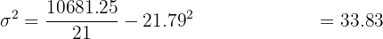
Variance
We calculate the sum of  , divide it by , and subtract the square of the arithmetic mean
  .
.

Standard Deviation
We take the square root of the variance:

Calculate the mean, median, and mode of the following series of numbers:

We create a table with the following columns:
- The values of the variable (
 )
) - The absolute frequencies ()
- The cumulative frequencies () to calculate the median
- The product of the variable by its absolute frequency () to calculate the mean
| Value | Frequency | Cumulative Frequency | fx |
|---|---|---|---|
| 2 | 2 | 2 | 4 |
| 3 | 2 | 4 | 6 |
| 4 | 5 | 9 | 20 |
| 5 | 6 | 15 | 30 |
| 6 | 2 | 17 | 12 |
| 8 | 3 | 20 | 24 |
| 20 | 96 |
Mode
The mode is the value with the highest absolute frequency. Looking at the column with values, the highest absolute frequency is 6, which corresponds to  .
.

Median
To calculate the median, we divide by 2, and we see that the cell with where 10 appears corresponds to .
Mean
We calculate the sum of the variable by its absolute frequency (), which is 96, and divide it by .

Find the variance and standard deviation of the following series of data:

We calculate the arithmetic mean:

We apply the variance formula:

We take the square root of the variance:

Find the mean, median, and mode of the following series of numbers:

Mode
The mode is 5 because it is the value that appears most frequently.

Median
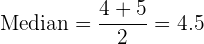
The series has an even number of values, so the median will be the average of the two central values.
Mean
We apply the mean formula.

Find the mean deviation, variance, and standard deviation of the following series of numbers:
1 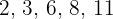
2 
1
Mean
Mean Deviation

Variance

Standard Deviation

2
Mean
Mean Deviation

Variance

Standard Deviation

A test was administered to factory employees, obtaining the following table:
| Interval | Frequency |
|---|---|
| [38, 44) | 7 |
| [44, 50) | 8 |
| [50, 56) | 15 |
| [56, 62) | 25 |
| [62, 68) | 18 |
| [68, 74) | 9 |
| [74, 80) | 6 |
Draw the histogram and the cumulative frequency polygon.
We add a new column with the cumulative frequencies ():
In the first cell we place the first absolute frequency.
In the second cell we add the value of the previous cumulative frequency plus the corresponding absolute frequency, and so on until the last, which must be equal to  .
.
| Interval | Frequency | Cumulative Frequency |
|---|---|---|
| [38, 44) | 7 | 7 |
| [44, 50) | 8 | 15 |
| [50, 56) | 15 | 30 |
| [56, 62) | 25 | 55 |
| [62, 68) | 18 | 73 |
| [68, 74) | 9 | 82 |
| [74, 80) | 6 | 88 |
| 88 |
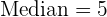
Given the statistical series:

Calculate:
- The mode, median, and mean
- The mean deviation, variance, and standard deviation
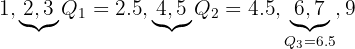
- Quartiles 1 and 3
- Deciles 2 and 7
- Percentiles 32 and 85
a 
Mode
There is no mode because all values have the same frequency.
Median
Ordering the data:
Therefore, the median is:
Mean

Variance

Standard Deviation

Mean Deviation

Range

Quartiles
Deciles
The formula for the position of deciles is:

Therefore, the deciles we are looking for are at positions:

Percentiles
The formula for the position of percentiles is:

Therefore, the percentiles we are looking for are at positions:

b 
Mode
There is no mode because all values have the same frequency.
Median
Ordering the data:
Therefore, the median is:
Mean

Variance

Standard Deviation

Mean Deviation

Range

Quartiles
Deciles
The formula for the position of deciles is:
Therefore, the deciles we are looking for are at positions:

Percentiles
The formula for the position of percentiles is:
Therefore, the percentiles we are looking for are at positions:

A statistical distribution is given by the following table:
| Interval | Frequency |
|---|---|
| [10, 15) | 3 |
| [15, 20) | 5 |
| [20, 25) | 7 |
| [25, 30) | 4 |
| [30, 35) | 2 |
Calculate:
- The mode, median, and mean.
- The range, mean deviation, and variance.
- Quartiles 1 and 3.
- Deciles 3 and 6.
- Percentiles 30 and 70.
We complete the table with:
- The cumulative frequency () to calculate the median
- The product of the variable by its absolute frequency () to calculate the mean
- The deviation from the mean and its product by the absolute frequency to calculate the mean deviation
- The product of the variable squared by its absolute frequency () to calculate the variance
| Interval | Frequency | Cumulative Frequency | fx | f(x - Mean)² | fx² | |
|---|---|---|---|---|---|---|
| [10, 15) | 12.5 | 3 | 3 | 37.5 | 27.857 | 468.75 |
| [15, 20) | 17.5 | 5 | 8 | 87.5 | 21.429 | 1537.3 |
| [20, 25) | 22.5 | 7 | 15 | 157.5 | 5 | 3543.8 |
| [25, 30) | 27.5 | 4 | 19 | 110 | 22.857 | 3025 |
| [30, 35) | 32.5 | 2 | 21 | 65 | 21.429 | 2112.5 |
| 21 | 457.5 | 98.571 | 10681.25 |
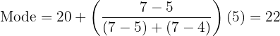
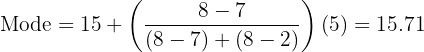
Mode
First, we find the interval where the mode is located, which will be the interval with the highest absolute frequency ().
Modal class: 
We apply the formula for calculating the mode for grouped data, extracting the following data:
Lower limit: 


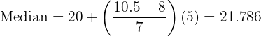
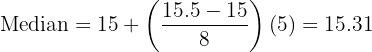
Median
We find the interval where the median is located by dividing by 2, since the median is the central value:

We look in the column of cumulative frequencies () for the interval that contains 10.5:
Median class:
We apply the formula for calculating the median for grouped data, extracting the following data:


Mean
We calculate the sum of the variable by its absolute frequency (), which is 457.5, and divide it by  :
:

Range
We find the difference between the largest and smallest values:

Mean Deviation
We calculate the sum of the products of deviations from the mean by their corresponding absolute frequencies , which is 98.571, and divide by :

Variance
We calculate the sum of  , divide it by , and subtract the square of the arithmetic mean .
Quartiles
Calculation of the first quartile
We find the interval where the first quartile is located by multiplying 1 by and dividing by 4:

We look in the column of cumulative frequencies () for the interval that contains 5.25:
Class of  :
: 
We apply the formula for calculating quartiles for grouped data, extracting the following data:


Calculation of the third quartile
We find the interval where the third quartile is located by multiplying 3 by and dividing by 4:
We look in the column of cumulative frequencies () for the interval that contains 15.75:
Class of  :
: 
We apply the formula for calculating quartiles for grouped data, extracting the following data:


Deciles
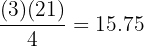
Calculation of the third decile
We find the interval where the third decile is located by multiplying 3 by and dividing by 10:

We look in the column of cumulative frequencies () for the interval that contains 6.3:
Class of  :
:
We apply the formula for calculating deciles for grouped data, extracting the following data:

Calculation of the sixth decile
We find the interval where the sixth decile is located by multiplying 6 by and dividing by 10:

We look in the column of cumulative frequencies () for the interval that contains 12.6:
Class of  :
:
We apply the formula for calculating deciles for grouped data, extracting the following data:


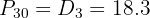
Percentiles
The 30th percentile is equal to the 3rd decile
Calculation of the 70th percentile
We find the interval where the 70th percentile is located by multiplying 70 by and dividing by 100:

We look in the column of cumulative frequencies () for the interval that contains 14.7:
Class of  :
:
We apply the formula for calculating percentiles for grouped data, extracting the following data:

Given the statistical distribution:
| Interval | Frequency |
|---|---|
| [0, 5) | 3 |
| [5, 10) | 5 |
| [10, 15) | 7 |
| [15, 20) | 8 |
| [20, 25) | 2 |
| [25, ∞) | 6 |
Find:
- The median and mode.
- Quartiles 1 and 3.
- Mean.
We extend the table with another column where we place the cumulative frequency ():
In the first cell we place the first absolute frequency.
In the second cell we add the value of the previous cumulative frequency plus the corresponding absolute frequency, and so on until the last, which must be equal to  .
.
| Interval | Value | Frequency | Cumulative Frequency |
|---|---|---|---|
| [0, 5 | 2.5 | 3 | 3 |
| [5, 10) | 7.5 | 5 | 8 |
| [10, 15) | 12.5 | 7 | 15 |
| [15, 20) | 17.5 | 8 | 23 |
| [20, 25) | 22.5 | 2 | 25 |
| [25, ∞) | 6 | 31 | |
| 31 |
Mode
First, we find the interval where the mode is located, which will be the interval with the highest absolute frequency ().
Modal class:
We apply the formula for calculating the mode for grouped data, extracting the following data:
Lower limit: 


Median
We find the interval where the median is located by dividing by 2, since the median is the central value:

We look in the column of cumulative frequencies () for the interval that contains 15.5:
Median class:
We apply the formula for calculating the median for grouped data, extracting the following data:
Quartiles
Calculation of the first quartile
We find the interval where the first quartile is located by multiplying 1 by and dividing by 4:

We look in the column of cumulative frequencies () for the interval that contains 7.75:
Class of : 
We apply the formula for calculating quartiles for grouped data, extracting the following data:


Calculation of the third quartile
We find the interval where the third quartile is located by multiplying 3 by and dividing by 4:

We look in the column of cumulative frequencies () for the interval that contains 23.25:
Class of :
We apply the formula for calculating quartiles for grouped data, extracting the following data:


Mean
The mean cannot be calculated because we cannot determine the class mark of the last interval.
If you want your children to reinforce this subject, or need to reinforce it yourself, don't hesitate to visit Superprof to find elementary school math classes or, if you prefer, an online math teacher.
Summarize with AI:
Did you like this article? Rate it!